Introduction
Simulation results are most useful when checked against measured performance in real homes. This case study compares a Solar Butter historic simulation for a Gloucester home against actual app readings from May to December 2025.
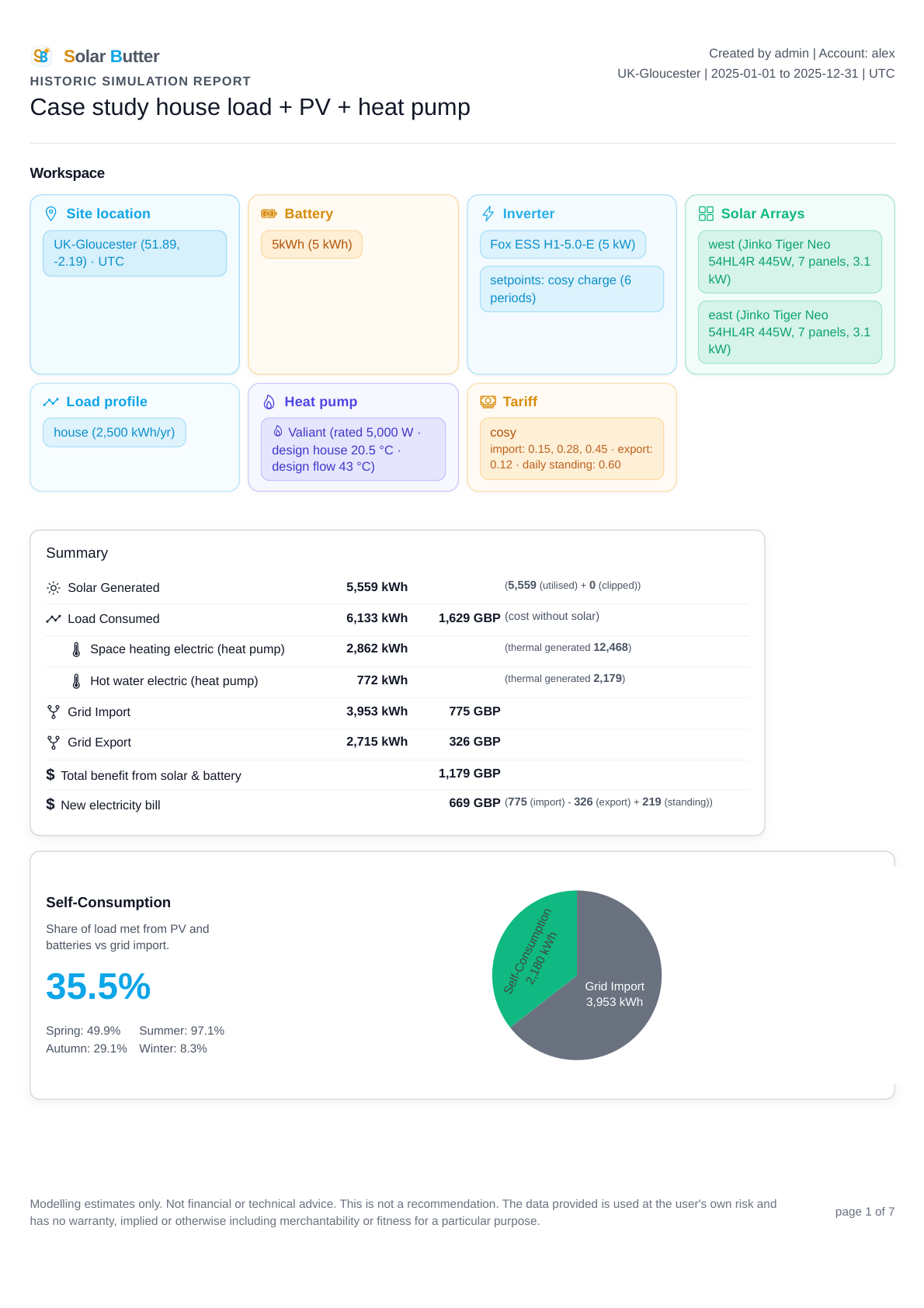
The home has an east/west PV array, battery storage, household load, and a Vaillant heat pump. The modelled values come from the hourly report CSV used to generate the calculator report, grouped by calendar month. The actual values come from the homeowner's PV, grid, load, and heat pump apps.
The calculator uses hour-by-hour historic weather data for the exact time period used in these scenarios.
These reports were modelled using our solar calculator: open the free Solar Butter solar calculator, which is free to use with no sign up required.
Assumptions
- Comparison period: May to December 2025
- Historic weather archive for the simulation period
- PV irradiance and solar position: pvlib (Holmgren et al., 2018), with a scalar shading factor applied to the array
- Model source: hourly Solar Butter historic report CSV, summed by calendar month
- Solar and grid metrics: PV generation, grid export, grid import, and total load
- Heat pump metric: electrical consumption comparison between modelled and actual
Results
9% high
The calculator modelled 4,092 kWh from May to December, against 3,771 kWh actual.
In line
The model predicted 1,648 kWh imported, against 1,654 kWh actual.
12% low
The modelled heat pump electricity was 1,532 kWh, against 1,736 kWh actual.
| Month | PV model / actual | Export model / actual | Import model / actual | Load model / actual | Heat pump electric model / actual |
|---|---|---|---|---|---|
| May | 809 / 850 | 497 / 534 | 50 / 14 | 356 / 315 | 144 / 134 |
| Jun | 843 / 799 | 568 / 517 | 11 / 8 | 281 / 277 | 76 / 112 |
| Jul | 783 / 745 | 512 / 491 | 0 / 13 | 267 / 253 | 55 / 99 |
| Aug | 662 / 651 | 388 / 381 | 10 / 28 | 280 / 284 | 68 / 114 |
| Sep | 473 / 450 | 236 / 187 | 125 / 101 | 358 / 356 | 153 / 158 |
| Oct | 267 / 167 | 28 / 10 | 335 / 304 | 445 / 457 | 233 / 229 |
| Nov | 152 / 72 | 0 / 0 | 511 / 515 | 581 / 584 | 376 / 387 |
| Dec | 103 / 37 | 0 / 0 | 606 / 672 | 650 / 703 | 437 / 503 |
| Metric | Calculator | Actual | Difference | Difference % |
|---|---|---|---|---|
| PV generation | 4,092 kWh | 3,771 kWh | +321 kWh | +9% |
| Grid export | 2,229 kWh | 2,120 kWh | +109 kWh | +5% |
| Grid import | 1,648 kWh | 1,654 kWh | -6 kWh | 0% |
| Load | 3,218 kWh | 3,228 kWh | -10 kWh | 0% |
| Heat pump electricity | 1,532 kWh | 1,736 kWh | -204 kWh | -12% |
Comparison
PV
Summer PV generation is close. From May to August, the calculator estimates 3,097 kWh and the home generated 3,045 kWh, only about 2% high. September is also close: 473 kWh modelled against 450 kWh actual. Table 1 shows the same pattern across all months.
The main divergence appears in the low-output winter months. From October to December, the calculator estimates 522 kWh, while the home generated 276 kWh. That is a large percentage gap, but it is concentrated in months where the absolute solar yield is already small.
This gap can be explained by site-specific shading and the large trees to the south of the property. These trees only materially affect the array in winter, when the sun is lower in the sky, but at that time they significantly reduce the already small winter generation values. The roof also suffers from some winter shading. The panels do not have optimisers, which can increase output loss under partial shading on affected panels or strings (Sharma and Harinarayan, 2013).
The simulator currently applies a single shading factor to account for site-specific shading. It is clear from this example that shading can affect performance more severely in winter, and so 3D view factor modelling should be considered as an improvement option in the future.
Heat pump
This comparison relies on an accurate site survey and heat loss calculation of the property. Heat loss surveys typically over-estimate heat loss on the side of caution (MCS, 2023), so we are more concerned with the trends in the data rather than the absolute values.
The heat pump electricity values are reasonably close. Across May to December, the calculator and actual values differ by around 12%, which is still a useful level of agreement for annual electricity planning. Table 1 shows the seasonal increase in heat pump electricity through the colder months.
The model captures the expected trend: a large increase in heat pump electricity demand in winter, associated with colder temperatures and lower COP.
Limitations
- Occupancy increased in September 2025, and the homeowner used slightly different setpoints (for example, house temperature) throughout the year.
- Shading is represented by a scalar factor, not time-varying obstructions such as trees or roof geometry.
- No independent calibration of monitoring hardware accuracy was performed.
Conclusion
The calculator gave a credible estimate of PV generation, export, total load direction, and total heat pump electrical demand.
The biggest visible mismatch is winter PV generation, where unmodelled trees and roof shading reduce the measured output compared with the simulation.
Overall, the model is close across the May–December electricity metrics in Table 2, while highlighting why local shading assumptions matter for low-output months.
References
- Holmgren, W.F., Hansen, C.W. and Mikofski, M.A. (2018) 'pvlib python: a python package for modeling solar energy systems', Journal of Open Source Software, 3(29), p. 884. doi:10.21105/joss.00884.
- IEA PVPS Task 16 (2018) Best Practice Guidelines for the Validation of Solar Simulation Models. IEA PVPS T16-04:2018.
- MCS (2023) MIS 3005 Issue 5.1: Heat Pump Design and Installation. Microgeneration Certification Scheme.
- Sharma, V. and Harinarayan, A. (2013) 'Impact of partial shading on solar PV module output characteristics', Renewable Energy, 55, pp. 374–382.